Many interesting problems in machine learning are being revisited with new deep learning tools. For graph-based semi-supervised learning, a recent important development is graph convolutional networks (GCNs), which nicely integrate local vertex features and graph topology in the convolutional layers. Although the GCN model compares favorably with other state-of-the-art methods, its mechanisms are not clear.
In our paper,
Li et al. (AAAI 2018), Deeper Insights into Graph Convolutional Networks for Semi-Supervised Learning
we develop deeper insights into the GCN model and address its fundamental limits. First, we show that the graph convolution of the GCN model is actually a special form of Laplacian smoothing, which is the key reason why GCNs work, but it also brings potential concerns of oversmoothing with many convolutional layers. Second, to overcome the limits of the GCN model with shallow architectures, we propose both co-training and self-training approaches to train GCNs. Our approaches significantly improve GCNs in learning with very few labels, and exempt them from requiring additional labels for validation. Extensive experiments on benchmarks have verified our theory and proposals.
Semi-supervised Classification Problem
A graph is represented by \(\mathcal{G}=(\mathcal{V},\mathcal{E})\), where \(\mathcal{V}\) is the vertex set with \(|\mathcal{V}| = n\) and \(\mathcal{E}\) is the edge set. We consider undirected graphs. Denote by \(A=[a_{ij}]\in{\mathbb R}^{n\times n}\) the adjacency matrix which is nonnegative. Each vertex \(i\) also has a \(c\)-dimensional feature vector \(\mathbf{x}_i \in R^{c}\). By stacking all feature vectors vertically, we obtain a feature matrix \(X=[\mathbf{x}_1,\mathbf{x}_2,\cdots,\mathbf{x}_n]^\top \in R^{n\times c}\). The problem we consider is semi-supervised classification on graphs.
Suppose that vertices are divided into two mutual exclusive subsets, a small labeled set \(\mathcal{V}_l\) and a large unlabeled set \(\mathcal{V}_u\), and labels of vertices in \(\mathcal{V}_l\) are given, the goal is to predict the labels of the remaining unlabeled vertices via graph structure \(A\) and vertex features \(X\).
Graph Convolutional Networks
Graph Convolutional Networks was proposed by Kipf & Welling. This model contains the following steps:
-
Construct the convolutional filter from adjacency matrix \(A\) by 1) adding an extra self-loop to each vertex, which results in a new adjacency matrix \(\tilde{A}=A+I\) an a new degree matrix \(\tilde{D}=D+I\), 2) then normalizing it and get the filter \(\hat{A}=\tilde{D}^{-\frac12}\tilde{A}\tilde{D}^{-\frac12}\).
-
Define the propagation rule for the graph convolutional layer \[ H^{(t+1)}= \sigma \left(\hat{A}H^{(t)}\Theta^{(t)}\right), \] where \(H^{(t)}\) is the matrix of activations in the \(t\)-th layer and \(H^{(0)} = X\), \(\Theta^{(t)}\) is the trainable weight matrix in layer \(t\), and \(\sigma\) is the activation function, e.g., \(\text{ReLU}(\cdot) = \max(0, \cdot)\). Theis graph convolution is defined by multiplying the input of each layer with the renormalized adjacency matrix \(\tilde{A}\) from the left, i.e., \(\tilde{A}H^{(t)}\). The convoluted representation of vertices are then fed into a standard fully-connected layers.
-
Stack two layers up and apply a softmax function on the output features to produce a prediction matrix: \[ Z = \text{softmax}\left ( \tilde{A}\; \text{ReLU}\left( \tilde{A}X\Theta^{(0)} \right)\Theta^{(1)} \right), \] and train the model using the cross-entropy loss over the labeled instances.
The key is the convolutional.
To understand the reasons why GCNs work so well, we compare them with the simplest fully-connected networks (FCNs), where the layer-wise propagation rule is \[\begin{equation} H^{(l+1)} = \sigma \left( H^{(l)}\Theta^{(l)} \right ). \end{equation} \] Clearly the only difference between a GCN and a FCN is the appearances/disappearance of the convolution filter \(\hat{A}\). To see the impact of the graph convolution, we tested the performances of GCNs and FCNs for semi-supervised classification on the Cora citation network with 20 labels in each class. The results are shown in following table. Surprisingly, even a one-layer GCN outperformed a one-layer FCN by a very large margin.
| classification accuracy | MLP | GCN |
|---|---|---|
| 1-layer | 53.08% | 70.79% |
| 2-layer | 55.92% | 79.83% |
We will show that this convolution is actually a special form of Laplacian smoothing in the following part. This convolution computes a new representation for each vertex which is smoother (more close to its neighbors) than the original one. Since vertices in the same cluster tend to be densely connected, the smoothing makes their representations similar, which makes the subsequent classification task much easier. As we can see from above table, applying the smoothing only once has already led to a huge performance gain.
Laplacian Smoothing
How to smooth a curve, which contains a series of discrete points, \(p_i\)? A method is to move each point to the weighted mean of its neighbors by \[ p_i \leftarrow p_i + \frac12L(p_i), \] where \(L(p_i)=\frac{(p_{i+1} + p_{i-1})}{2}-p_i\). This operation may be performed iteratively.
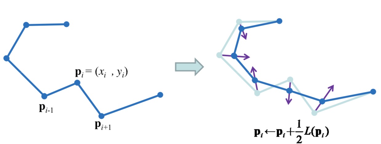 image via here
We now take curves as a graphs with an adjacency matrix \(A \) and \(a_{ij}=1\) iff \(|i-j|=1\). Denote by \(D=\mathrm{diag}(d_1,d_2,\ldots,d_n)\) the degree matrix of \(A\) where \(d_i=\sum_{j}a_{ij}\) is the degree of vertex \(i\). We can rewrite above smooth in matrix form \[ P\leftarrow (I - \frac12 L_{\mathrm{rw}})P, \] where \[P= \begin{bmatrix} x_1 & y_1 \\ x_2 & y_2 \\ \vdots & \vdots \\ x_n & y_n \\ \end{bmatrix} \quad L_{\mathrm{rw}}=\begin{bmatrix} 1 & -1 & \\ -\frac12 & 1 & -\frac12 \\ & \ddots & \ddots & \ddots \\ & & -\frac12 & 1 & -\frac12 \\ & & & -1 & 1 \\ \end{bmatrix} \]
Here \(L\) is actually normalized graph Laplacian. More formally, the graph Laplacian (Chung 1997) is defined as \(L=D-A\), and the two versions of normalized graph Laplacians are defined as \(L_{\mathrm{sym}}:=D^{-\frac{1}{2}}LD^{-\frac{1}{2}}\) and \(L_{\mathrm{rw}}: = D^{-1}L\) respectively. The Laplacian smoothing is \[ P\leftarrow (I - \gamma L_{\mathrm{rw}})P. \] Here \(0\le \gamma \le 1\) controls the strength of smoothing.
If we let \(\gamma=1\) and replace the \(L_{\mathrm{rw}}\) with \(L_{\mathrm{sym}}\), then this smoothing method is exactly the convolution used by GCNs. The Laplacian smoothing computes the local average of each vertex as its new representation. Since vertices in the same cluster tend to be densely connected, the smoothing makes their features similar, which makes the subsequent classification task much easier. This is the reason why GCNs work.
Summary
Understanding deep neural networks is crucial for realizing their full potentials in real applications. Our paper contributes to the understanding of the GCN model and its application in semi-supervised classification. Our analysis not only reveals the mechanisms and but also the limitations of the GCN model. Laplacian suffers from shrinkage problem, which leads to the oversmoothing problem of GCNs. We also derived solutions from our analysis to overcome its limits. See our paper for more details. If you have any question, please email me.